Tutorial 5: Colors and colorbars

This tutorial demonstrates how to configure the colorbar(s) with surfplot.

Layer color maps and colorbars

The color map can be specified for each added plotting layer using the cmap parameter of add_layer(), along with the associated matplotlib colorbar drawn if specified. The colobar can be turned off by cbar=False. The range of the colormap is specified with the color_range parameter, which takes a tuple of (minimum, maximum) values. If no color range is specified (the default, i.e. None), then the color range is computed automically based on the minimum and maximum of the data.

Let’s get started by setting up a plot with surface shading added as well. Following the first initial steps of Tutorial 1: Quick Start :

from neuromaps.datasets import fetch_fslr
from surfplot import Plot

surfaces = fetch_fslr()
lh, rh = surfaces['inflated']
p = Plot(lh, rh)

sulc_lh, sulc_rh = surfaces['sulc']
p.add_layer({'left': sulc_lh, 'right': sulc_rh}, cmap='binary_r', cbar=False)

Now let’s add a plotting layer with a colorbar using the example data. The cmap parameter accepts any named matplotlib colormap, or a colormap object. This means that surfplot can work with pretty much any colormap, including those from seaborn and cmasher, for example.

from surfplot.datasets import load_example_data

# default mode network associations
default = load_example_data(join=True)
p.add_layer(default, cmap='GnBu_r', cbar_label='Default mode')
fig = p.build()
fig.show()

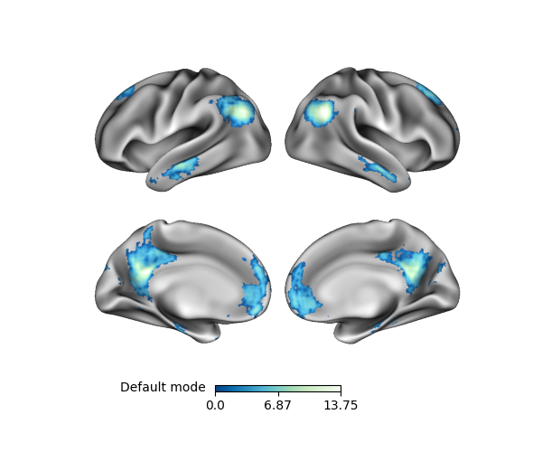
cbar_label added a text label to the colorbar. Although not necessary in cases where a single layer/colorbar is shown, it can be useful when adding multiple layers. To demonstrate that, let’s add another layer using the frontoparietal network associations from load_example_data():

fronto = load_example_data('frontoparietal', join=True)
p.add_layer(fronto, cmap='YlOrBr_r', cbar_label='Frontoparietal')
fig = p.build()
fig.show()

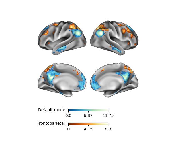
The order of the colorbars is always based on the order of the layers, where the outermost colorbar is the last (i.e. uppermost) plotting layer. Of course, more layers and colorbars can lead to busy-looking figure, so be sure not to overdo it.

cbar_kws

Once all layers have been added, the positioning and style can be adjusted using the cbar_kws parameter in build(), which are keyword arguments for surfplot.plotting.Plot._add_colorbars(). Each one is briefly described below (see _add_colorbars() for more detail):

1. location: The location, relative to the surface plot

2. label_direction: Angle to draw label for colorbars

3. n_ticks: Number of ticks to include on colorbar

4. decimals: Number of decimals to show for colorbal tick values

5. fontsize: Font size for colorbar labels and tick labels

6. draw_border: Draw ticks and black border around colorbar

7. outer_labels_only: Show tick labels for only the outermost colorbar

8. aspect: Ratio of long to short dimensions

9. pad: Space that separates each colorbar

10. shrink: Fraction by which to multiply the size of the colorbar

11. fraction: Fraction of original axes to use for colorbar

Let’s plot colorbars on the right, which will generate vertical colorbars instead of horizontal colorbars. We’ll also add some style changes for a cleaner look:

kws = {'location': 'right', 'label_direction': 45, 'decimals': 1,
       'fontsize': 8, 'n_ticks': 2, 'shrink': .15, 'aspect': 8,
       'draw_border': False}
fig = p.build(cbar_kws=kws)
fig.show()
# sphinx_gallery_thumbnail_number = 3

Be sure to check out Example 1: Multiple Stat Maps for another example of colorbar styling.

Transparency

The transparency of the plotting layers can be adjusted by the alpha parameter. This may be preferred in cases with overlapping plotting layers. We can recreate the example above with transparent maps like so:

p = Plot(lh, rh)
p.add_layer({'left': sulc_lh, 'right': sulc_rh}, cmap='binary_r', cbar=False)
p.add_layer(default, cmap='GnBu_r', cbar_label='Default mode', alpha=.5)
p.add_layer(fronto, cmap='YlOrBr_r', cbar_label='Frontoparietal', alpha=.5)
fig = p.build(cbar_kws=kws)
fig.show()

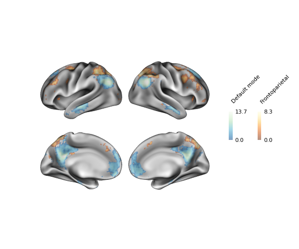
Although these particular maps are largely non-overlapping, you can see some small overlap at the edges of the default mode and frontoparietal clusters thanks to the transparency.