Tutorial 3: Types of Input Data

This tutorial covers what types of data can be passed to the data parameter of the add_layer() method of Plot.

data accepts four different types of data:

1. A numpy array of vertex data

2. A file path of a valid GIFTI or CIFTI file

3. Instances of nibabel.gifti.gifti.GiftiImage or nibabel.cifti2.cifti2.Cifti2Image

4. A dictionary with ‘left’ and/or ‘right’ keys to explicity assign any of the above data types to either hemisphere.

This flexibility makes it easy to plot any surface data by accommodating both GIFTI and CIFTI data. Let’s dig into this further.

Getting data

Here we’ll reuse the Conte69 fsLR surfaces and Freesurfer sulc maps we used in Tutorial 1: Quick Start, both of which are downloaded via neuromaps. We’ll also reuse the example data.

from neuromaps.datasets import fetch_fslr
from surfplot.datasets import load_example_data

surfaces = fetch_fslr()
lh, rh = surfaces['inflated']

Arrays

A numpy array can be passed to data in the add_layer() method. Importantly, the length of this array must equal the total number of vertices of the hemispheres that are plotted. With our surfaces, we can check their vertices using nibabel:

import nibabel as nib
print('left', nib.load(lh).darrays[0].dims)
print('right', nib.load(rh).darrays[0].dims)

left [32492, 3]
right [32492, 3]

Therefore, our data must have a length of 32492 + 32492 = 64984 if we want to plot both hemispheres. Let’s check this first:

# return a single concatenated array from both hemispheres
data = load_example_data(join=True)
print(len(data) == 64984)

True

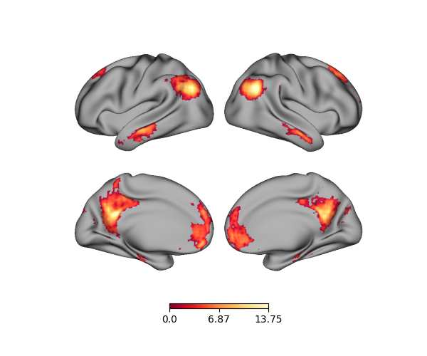
Perfect, now let’s plot:

from surfplot import Plot

p = Plot(surf_lh=lh, surf_rh=rh)
p.add_layer(data, cmap='YlOrRd_r')
fig = p.build()
fig.show()

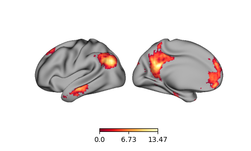
Note that passing a single array assumes it goes from the left hemisphere to the right. If we want to plot just one hemisphere, then we have to update our data accordingly. Be sure to plot the correct data!

p = Plot(surf_lh=lh, zoom=1.2, size=(400, 200))
# left hemisphere is the first 32492 vertices
p.add_layer(data[:32492], cmap='YlOrRd_r')
fig = p.build()
fig.show()
# sphinx_gallery_thumbnail_number = 2

Using a dictionary

To be explicit about which data is passed to which hemisphere, it is also possible to use a dictionary to assign data to a hemisphere. The dictionary must have ‘left’ and/or ‘right’ keys only. This is exactly how data was passed to the final figure in Tutorial 1: Quick Start. Note that the length of each array must equal the number of vertices in their respective hemispheres.

# return as separate arrays for each hemisphere
lh_data, rh_data = load_example_data()

p = Plot(surf_lh=lh, surf_rh=rh)
p.add_layer({'left': lh_data, 'right': rh_data}, cmap='YlOrRd_r')
fig = p.build()
fig.show()

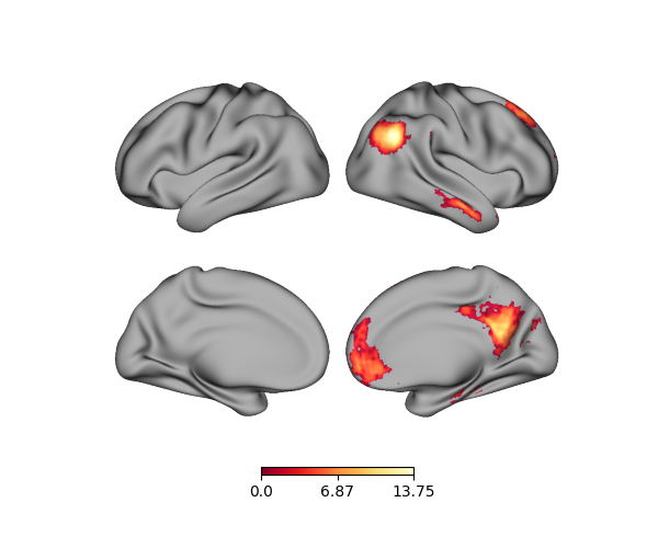
Using a dictionary, we can also only plot data for a specific hemisphere, e.g., the right:

p = Plot(surf_lh=lh, surf_rh=rh)
p.add_layer({'right': rh_data}, cmap='YlOrRd_r')
fig = p.build()
fig.show()

Using dictionaries is necessary when plotting data from left and/or right GIFTI files, which we’ll cover in the next section.

File names

It is possible to directly pass in file names, assuming that they’re valid and readable with nibabel. These files must be either GIFTI or CIFTI images. When plotting both hemispheres, you will need a dictionary to assign each each GIFTI to a hemisphere. To test this out, let’s get the downloaded sulc maps and add them:

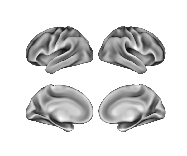
lh_sulc, rh_sulc = surfaces['sulc']
p = Plot(surf_lh=lh, surf_rh=rh)
p.add_layer({'left': lh_sulc, 'right': rh_sulc}, cmap='binary_r', cbar=False)
fig = p.build()
fig.show()

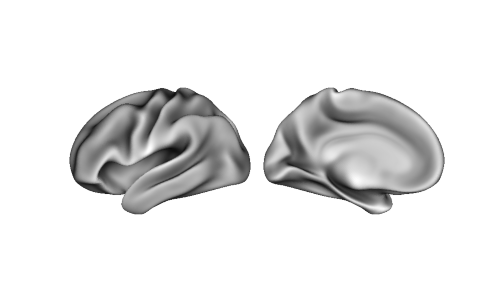
Loaded files

Finally, if a file was already loaded into Python using nibabel, then it can also be plotted. For example, with single hemisphere:

img = nib.load(lh_sulc)

p = Plot(surf_lh=lh, zoom=1.2, size=(400, 200))
p.add_layer(img, cmap='binary_r', cbar=False)
fig = p.build()
fig.show()

Altogether, this flexibility makes it easy to plot data in a variety of different workflows and usecases. As always, be sure to check that the data is passed to the correct hemisphere, and that the number of vertices in the data match the number of vertices of the surface(s)!