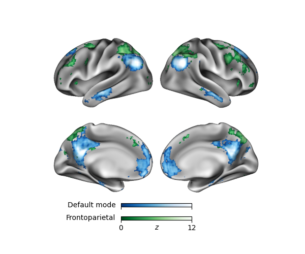
Example 1: Multiple Stat Maps

This example shows multiple statistical maps on a surface with some extra stylizing for a clean-looking figure.

# Code source: Dan Gale
# License: BSD 3 clause

from surfplot import Plot
from surfplot.datasets import load_example_data
from neuromaps.datasets import fetch_fslr

surfaces = fetch_fslr()
lh, rh = surfaces['inflated']

p = Plot(lh, rh)

# shading
lh_sulc, rh_sulc = surfaces['sulc']
p.add_layer({'left': lh_sulc, 'right': rh_sulc}, cmap='binary_r', cbar=False)

color_range = (0, 12)

# add default mode association stats
default = load_example_data(join=True)
p.add_layer(default, cmap='Blues_r', color_range=color_range,
            cbar_label='Default mode')

# add frontoparietal assocation stats
fronto = load_example_data('frontoparietal', join=True)
p.add_layer(fronto, cmap='Greens_r', color_range=color_range,
            cbar_label='Frontoparietal')

# create a clean looking set of colorbars. Only show labels for outer colorbar,
# given that both colorbars have the same range.
cbar_kws = dict(outer_labels_only=True, pad=.02, n_ticks=2, decimals=0)
fig = p.build(cbar_kws=cbar_kws)
# add units to colorbar
fig.axes[1].set_xlabel('z', labelpad=-11, fontstyle='italic')
fig.show()