Tutorial 1: Quick Start

This tutorial gives a quick overview of surfplot before diving into more detail in subsequent tutorials. The aim here is to get a flavour of how surfplot works and what can be plotted.

Getting surfaces

First, we need to get some brain surfaces. Here, we’ll use the Conte69 Human Connectome Project surface (A.K.A fsLR surfaces). We can import and call the neuromaps.datasets.fetch_fslr() function, and then select the ‘inflated’ surface, which will give the file paths of the left and right hemisphere GIFTI files:

from neuromaps.datasets import fetch_fslr

surfaces = fetch_fslr()
lh, rh = surfaces['inflated']

Making a plot

Brain plots are created using the brainspace.plotting.Plot class. We can pass both of our surfaces to the surf_lh and surf_rh parameters. These parameters accept file paths/names, or preloaded surfaces from brainspace.mesh.mesh_io.read_surface().

Then, we can call build() method to make the figure, which returns a matplotlib figure, fig.

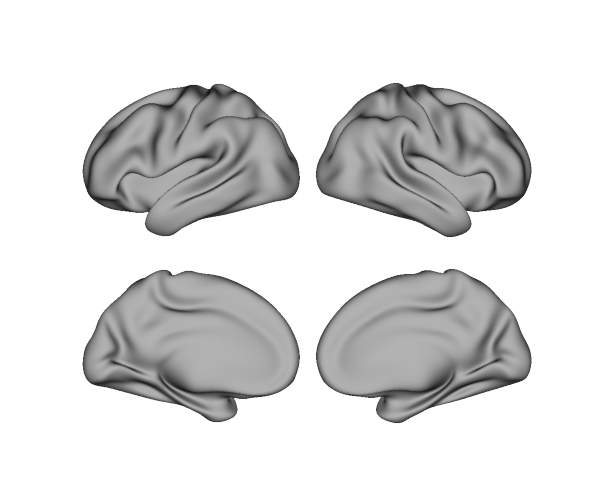
from surfplot import Plot

p = Plot(surf_lh=lh, surf_rh=rh)
fig = p.build()
# show figure, as you typically would with matplotlib
fig.show()

Adding layers

Once the plot has been set up by instantiating the Plot class, adding data is as simple as adding plotting layers using the add_layer() method.

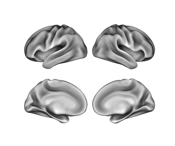
Let’s first add some shading. We already have the Freesurfer sulc maps in our surface variable, which are accessed here with the ‘sulc’ key.

We can pass our sulc maps to the add_layer() method with the first positional parameter, data, which accepts either a dictionary with ‘left’ and ‘right’ keys, or a numpy array. Tutorial 3: Types of Input Data covers what types of data can be passed to the data parameter.

sulc_lh, sulc_rh = surfaces['sulc']
p.add_layer({'left': sulc_lh, 'right': sulc_rh}, cmap='binary_r', cbar=False)

Above, we’ve also used a grayscale colormap (cmap) and turned off the colorbar (cbar) for this particular layer.

Now, let’s plot our updated figure:

fig = p.build()
fig.show()

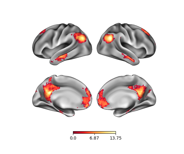
Finally, let’s add some statistical data. We can load some example data packaged with surfplot using load_example_data(). By default, it loads an association map of the term ‘default mode’ computed from Neurosynth. For convenience, this map has already been projected from a volume in MNI152 coordinates to a fsLR surface using neuromaps, and the lh_data and rh_data variables are just numpy arrays of the vertices:

from surfplot.datasets import load_example_data
lh_data, rh_data = load_example_data()
print(lh_data)

[6.6808 0.     0.     ... 0.     0.     0.    ]

We can add each array as a layer using a dictionary like before. By default a colorbar will be added for this layer, and its range is determined by the minimum and maximum values (this can be adjusted with the color_range parameter).

p.add_layer({'left': lh_data, 'right': rh_data}, cmap='YlOrRd_r')
fig = p.build()
fig.show()
# sphinx_gallery_thumbnail_number = 3