Tutorial 4: Layouts and Views

This tutorial covers the layout and view options provided by surfplot.

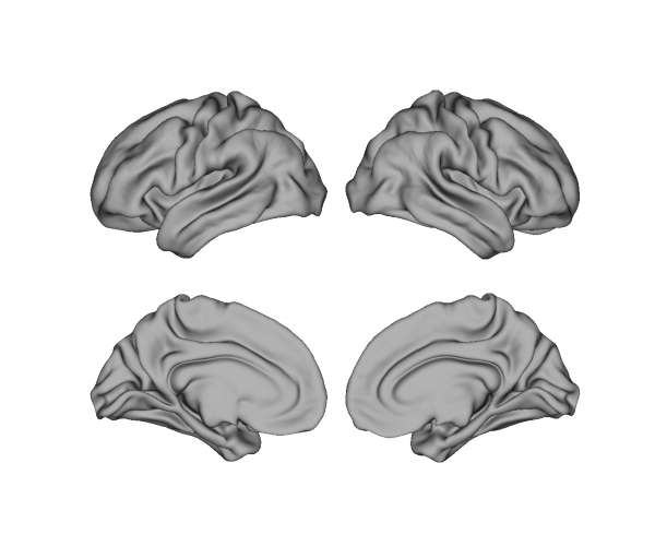
For variety, let’s import the left and right Conte69 midthickness surface directly using load_conte69(). Then, we’ll make a blank surface plot using the default layout and view, which is a 2x2 ‘grid’ of lateral and medial views that is identical to the default setup in Connectome Workbench.

from brainspace.datasets import load_conte69
from surfplot import Plot

lh, rh = load_conte69()
p = Plot(lh, rh)
fig = p.build()
fig.show()

Layout

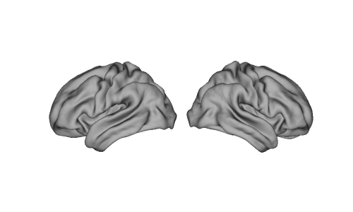
The layout can be adjusted with the layout parameter, and has 3 options: ‘grid’ (default, shown above), ‘row’, or ‘column’. The size and zoom parameters will have to be adjusted based on the layout and number of views.

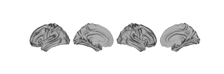
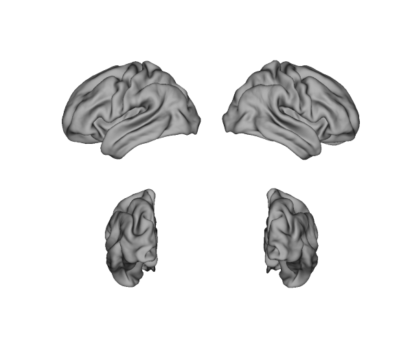
Above we see that ‘grid’ gives us a views-by-hemisphere grid, where the left hemisphere is the left column and the right hemisphere is the right column. Meanwhile, the ‘row’ layout gives a single horizontal row of brains:

p = Plot(lh, rh, size=(800, 200), zoom=1.2, layout='row')
fig = p.build()
fig.show()

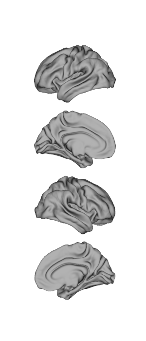
The ‘column’ layout gives a single vertical column of brains.

p = Plot(lh, rh, size=(200, 600), zoom=1.6, layout='column')
fig = p.build()
fig.show()
# sphinx_gallery_thumbnail_number = 3

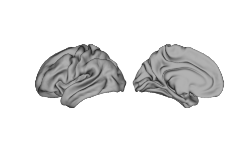
As well, it’s also possible to plot just one hemisphere. If the layout is set as default (‘grid’), then a single hemisphere is plotted as row:

p = Plot(lh, size=(400, 200), zoom=1.2)
fig = p.build()
fig.show()

Views

surfplot makes it easy to configure the view(s) you wish to use. One or more views can be specified through the views parameter. As we’ve seen before, the default is to include lateral and medial views. It is also possible to show just one view:

p = Plot(lh, rh, size=(400, 200), zoom=1.2, views='lateral')
fig = p.build()
fig.show()

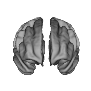
It is also possible to show more than just lateral and medial views, such as ‘posterior’. Note that views are plotted in order in which they appear in the list:

p = Plot(lh, rh, size=(500, 400), zoom=1.4,  views=['lateral', 'posterior'])
fig = p.build()
fig.show()

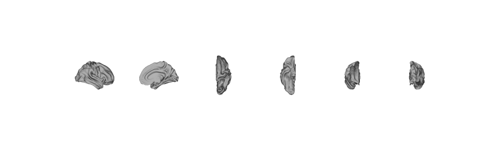
All possible views are shown here (the right hemisphere for brevity):

all_views = ['lateral', 'medial', 'dorsal', 'ventral', 'anterior', 'posterior']
p = Plot(surf_rh=rh, size=(900, 200), zoom=.8, layout='row', views=all_views)
fig = p.build()
fig.show()

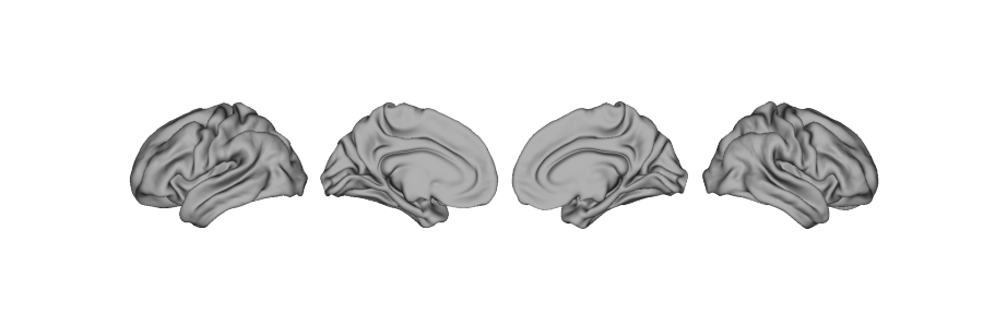
Views can also be mirrored when both hemipsheres are plotted and layout is either ‘row’ or ‘column’. Specifically, the right hemisphere view order is reversed. For example, plotting default lateral and medial views and setting mirror_views=True will situate the medial views in the middle for a symmetrical figure:

p = Plot(lh, rh, size=(800, 200), zoom=1.2, layout='row', mirror_views=True)
fig = p.build()
fig.show()

Finally, it is possible to flip the left and right hemisphere. This is useful when plotting just the ‘anterior’ or ‘ventral’ for both hemispheres. For example:

p = Plot(lh, rh, size=(200, 200), zoom=3, views='anterior', flip=True)
fig = p.build()
fig.show()