Note
Click here to download the full example code
Tutorial 6: Regions and Parcellations
This tutorial demonstrates how to plot brain regions.
Regions and parcellations can be plotted with brainplot as one or more
layers, and it’s possible to add region outlines by simply adding a layer with
the as_outline parameter.
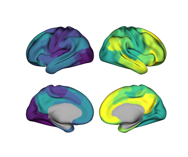
Parcellations
Multiple brain regions can be plotted as a single layer as long as the vertices
in different regions have different numerical labels/values, which is typical
for any parcelation. To demonstrate, we can use the
load_parcellation() from Brainspace to load the
Schaefer 400 parcellation.
from neuromaps.datasets import fetch_fslr
from surfplot import Plot
from brainspace.datasets import load_parcellation

surfaces = fetch_fslr()
lh, rh = surfaces['inflated']
p = Plot(lh, rh)

# add schaefer parcellation (no color bar needed)
lh_parc, rh_parc = load_parcellation('schaefer')
p.add_layer({'left': lh_parc, 'right': rh_parc}, cbar=False)

fig = p.build()
fig.show()
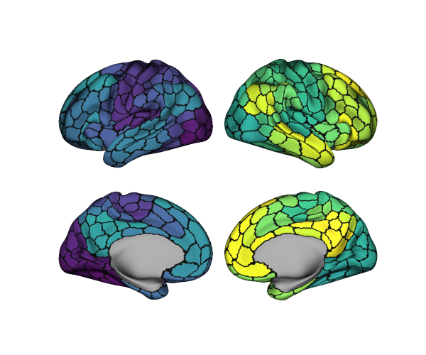
Now can add a second layer of just the region outlines. This is done by setting as_outline=True. The color of the outlines are set by the cmap parameter, as with any data. To show black outlines, we can just use the gray colormap.
p.add_layer({'left': lh_parc, 'right': rh_parc}, cmap='gray',
            as_outline=True, cbar=False)
fig = p.build()
fig.show()
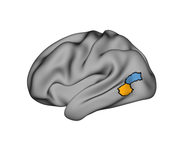
Regions of Interest
Often times we want to show a selection of regions, instead of all regions. These could be regions from a parcellation, regions defined from a functional localizer, etc.
Let’s select two regions from the Schaefer parcellation and zero-out the remaining regions. We’ll just stick with the left hemisphere here.
import numpy as np
region_numbers = [71, 72]
# zero-out all regions except 71 and 72
regions = np.where(np.isin(lh_parc, region_numbers), lh_parc, 0)
Although we can use a pre-defined color map, we might want to define a
custom colormap where we can define the exact color for each region. This is
possible using matplotlib:
from matplotlib.colors import ListedColormap

colors = ['orange', 'steelblue']
cmap = ListedColormap(colors, 'regions', N=2)
Now we can plot both regions with their outlines: only need to show the left lateral view
p = Plot(lh, views='lateral')
p.add_layer(regions, cmap=cmap, cbar=False)
p.add_layer(regions, cmap='gray', as_outline=True, cbar=False)

fig = p.build()
fig.show()
# sphinx_gallery_thumbnail_number = 3
Note
Multiple regions can also be plotted as individual layers, rather than combined as a single layer, as shown here. In this case, the vertex array(s) for each layer would be binary.
Total running time of the script: ( 0 minutes 0.506 seconds)